Computing the Kalman Filter connecting pieces
The Kalman Filter is an algorithm to update probability distributions with new observations made under noisy conditions. It is used in everything from smartphone GPS navigation systems to large scale climate simulations. It is implemented in hardware ranging from embedded devices to super-computers. It is important and widely used.
In this post I will
- Show how to compute the Kalman Filter with BLAS/LAPACK
- Relate this to old work on
sympy.stats - Analyze the computation graph for some flaws and features
Results
The Kalman filter can be defined as a pair of matrix expressions
# kalman.py
from sympy.matrices.expressions import MatrixSymbol, Identity
from sympy import Symbol, Q

n, k    = Symbol('n'), Symbol('k')
mu      = MatrixSymbol('mu', n, 1)
Sigma   = MatrixSymbol('Sigma', n, n)
H       = MatrixSymbol('H', k, n)
R       = MatrixSymbol('R', k, k)
data    = MatrixSymbol('data', k, 1)
I       = Identity(n)

new_mu      = mu + Sigma*H.T * (R + H*Sigma*H.T).I * (H*mu - data)
new_Sigma   = (I - Sigma*H.T * (R + H*Sigma*H.T).I * H) * Sigma

assumptions = (Q.positive_definite(Sigma) & Q.symmetric(Sigma) &
               Q.positive_definite(R) & Q.symmetric(R))
We convert these matrix expressions into a computation
# kalman_computation.py
from kalman import new_mu, new_Sigma, assumptions
from sympy.computations.matrices.compile import make_rule, patterns
from sympy.computations.core import Identity

ident = Identity(new_mu, new_Sigma)
rule = make_rule(patterns, assumptions)
mathcomp = next(rule(ident))
mathcomp.show()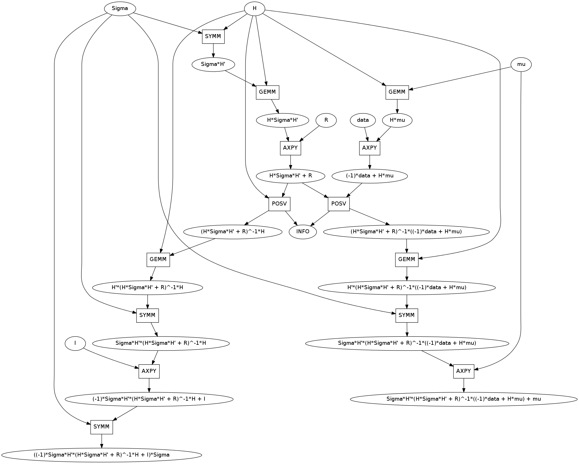
This is a useful result.
History with stats
Two years ago I wrote two blogposts about the Kalman filter, one on the univariate case and one on the multivariate case. At the time I was working on sympy.stats, a module that enabled uncertainty modeling through the introduction of a random variables into the SymPy language.
SymPy stats was designed with atomicity in mind. It tried to be as small and thin a layer as possible.
- It turned queries on continuous random expressions into integral expressions.
- It turned queries on discrete random expressions into iterators and sums.
- It also turned queries on multivariate normal random expressions into matrix expressions.
The goal was to turn a specialized problem (uncertainty quantification) into a general one (integrals, sums, matrix expressions) under the assumption that tools are much richer to solve general problems than specific ones.
The first blogpost on the univariate kalman filter produced integral expressions that were then solved by SymPy’s integration routines. The second blogpost on the multivariate Kalman filter generated the following matrix expressions
\(\mu' = \mu + \Sigma H^T \left( R + H \Sigma H^T \right )^{-1} \left(H\mu - \textrm{data} \right)\) \(\Sigma' = \left( \mathbb{I} - \Sigma H^T \left(R + H \Sigma H^T \right)^{-1} H \right) \Sigma\)
That blogpost finished with this result, claiming that the job of sympy.stats was finished and that any of the popular numerical linear algebra packages could pick up from that point.
These two equations are the Kalman filter and were our starting point for today. Matrix Expressions are an intermediate representation layer between sympy.stats and sympy.computations.matrices.
By composing these projects we compile high level statistical expressions of sympy.stats to intermediate level matrix expressions to the DAGs of sympy.computations and even down to low level Fortran code. If we add a traditional Fortran compiler we can build working binaries directly from sympy.stats.
Features and Flaws in the Kalman graph
Lets investigate the Kalman computation. It contains a few notable features.
First, unlike previous examples it has two outputs, new_mu and new_Sigma. These two have large common subexpressions like H*Sigma*H' + R. You can see that these were computed once and shared.
Second, lets appreciate that H*Sigma*H + R is identified as symmetric positive definite allowing the more efficient POSV routine. I’ve brought this up before in artificial examples. It’s nice to see that this occurs in practice.
Third, there is an unfortunately common motif. This instance was taken from the upper right of the image but the GE/SYMM -> AXPY motif occurs four times in this graph.
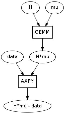
GEMM/SYMM are matrix multiply operations used to break down expressions like alpha*A*B. AXPY is a matrix addition used to break down expressions like alpha*A + B. They are both used properly here.
This motif is unforunate because GEMM is also capable of breaking down a larger expression like alpha*A*B + beta*C, doing a fused matrix multiply and add all in one pass. The AXPY would be unnecessary if the larger GE/SYMM patterns had matched correctly.
Canonicalization
The alpha*A*B + beta*C patterns did not match here for a silly reason, there wasn’t anything to match for the scalars alpha and beta. Instead the patterns were like A*B - C. One solution to this problem is to make more patterns with all possibilities. Alternatively we could change how we canonicalize MatMul objects so that they always have a scalar coefficient, even if it defaults to 1.
We don’t want to change MatMul to behave like this throughout all of SymPy though; the extra 1 is usually unwanted. This is a case where there are multiple correct definitions of canonical. Fortunately MatMul is written with this eventuality in mind.
Links
- A Lesson in Data Assimilation using SymPy
- Multivariate Normal Random Variables
- Source for this post: kalman.py, kalman_comp.py
blog comments powered by Disqus