Characteristic Functions and sympy.stats

In a recent post, Characteristic Functions and scipy.stats, Josef Perktold created functions for the characteristic functions of the Normal (easy) and t (hard) distributions. The t-distribution is challenging because the solution involves special functions and has numerically challenging behavior around 0 for high degrees of freedom. Some quotes

The characteristic function for the normal distribution is easy, but looking at the characteristic function of the t-distribution, I wish someone had translated it into code already

Since I haven’t seen it yet, I sat down and tried it myself. I managed to code the characteristic function of the t-distribution, but it returns NaNs when it is evaluated close to zero for large df. I didn’t find a Bessel “k” function that works in this case

He then includes his code and discusses a particular application of the characteristic function which I won’t discuss here.

Symbolic Solution

Josef wished that this code had been written already. Characteristic functions aren’t built into SymPy but we may be able to derive them automatically.

Wikipedia says that the characteristic function \(\phi(t)\) of a random variable X is defined as follows

It equal to the expectation of exp(i*t*X). Lets do this in SymPy

>>> from sympy.stats import *
>>> mu = Symbol('mu', bounded=True)
>>> sigma = Symbol('sigma', positive=True, bounded=True)
>>> t = Symbol('t', positive=True)

>>> X = Normal('X', mu, sigma)  # Normal random variable
>>> simplify(E(exp(I*t*X)))     # Expectation of exp(I*t*X)
              2  2
             σ ⋅t
     ⅈ⋅μ⋅t - ─────
               2
   ℯ

I was actually pretty surprised that this worked as smoothly as it did. SymPy stats wasn’t designed for this.

Here are some gists for the Cauchy and Student-T distributions. Cauchy simplifies down pretty well but the Student-T characteristic function has a few special functions included.

Behavior near zero

Josef says that the behavior of the characteristic function of the t distribution near zero for high degrees of freedom (the nu parameter) is challenging to compute numerically. Can SymPy handle this symbolically?

>>> nu = Symbol('nu', positive=True, integer=True)
>>> t = Symbol('t', positive=True)

>>> X = StudentT('X', nu)
>>> simplify(E(exp(I*t*X)))

The bold scripted I’s are besseli functions. We restrict this expression to a specific number of degrees of freedom, setting nu = 50

>>> simplify(E(exp(I*t*X))).subs(nu, 50)  # replace nu with 50
         ⎛         ___  ⎞            ⎛        ___  ⎞
∞⋅besseli⎝-25, 5⋅╲╱ 2 ⋅t⎠ - ∞⋅besseli⎝25, 5⋅╲╱ 2 ⋅t⎠

Whoops, simple substitution at that number of degrees of freedom fails, giving us infinities. What if we build the expression with 50 from the beginning? This gives the integration routines more information when they compute the expectation.

>>> X = StudentT('X', 50)
>>> simplify(E(exp(I*t*X)))
        ⎛              │     2  -ⅈ⋅π⎞           ⎛              │     2  ⅈ⋅π⎞
╭─╮3, 1 ⎜   1/2        │ 25⋅t ⋅ℯ    ⎟   ╭─╮3, 1 ⎜   1/2        │ 25⋅t ⋅ℯ   ⎟
│╶┐     ⎜              │ ───────────⎟ + │╶┐     ⎜              │ ──────────⎟
╰─╯1, 3 ⎝25, 0, 1/2    │      2     ⎠   ╰─╯1, 3 ⎝25, 0, 1/2    │     2     ⎠
────────────────────────────────────────────────────────────────────────────
                        1240896803466478878720000⋅π

The solution is in terms of Meijer-G functions. Can we evaluate this close to t = 0?

>>> simplify(E(exp(I*t*X))).subs(t, 1e-6).evalf()
0.999999999999479 + 1.56564942264937e-29⋅ⅈ

>>> simplify(E(exp(I*t*X))).subs(t, 1e-30).evalf()
1.0 - 1.2950748484704e-53⋅ⅈ

This is where scipy’s special functions failed in Josef’s post, yielding infinity instead of 1.

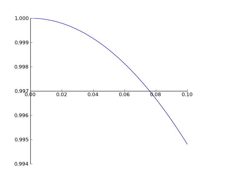
And finally we plot the behavior around 0.

>>> plot(re(simplify(E(exp(I*t*X)))), (t, 1e-7, 1e-1))

Closing Notes

The sympy.stats module was not designed with characteristic functions in mind. I was pleasantly surprised when I entered code almost identical to the mathematical definition

X = Normal('X', mu, sigma)
E(exp(I*t*X))

and received the correct answer. I am always happy when projects work on problems for which they were not originally designed. The fact that this works is largely due to SymPy’s excellent handling of integrals of special functions, due largely to Tom Bachmann.

If you do complex work on statistical functions I recommend you take a look at sympy.stats. It’s able to perform some interesting high level transformations. Thanks to recent work by Raoul Bourquin many of the common distributions found in scipy.stats are now available (with even more in a pull request).