Towards Out-of-core ND-Arrays -- Multi-core Scheduling
This work is supported by Continuum Analytics and the XDATA Program as part of the Blaze Project
tl;dr We show off a multi-threaded shared-memory task scheduler. We share two techniques for space-constrained computing. We end with pretty GIFs.
Disclaimer: This post is on experimental buggy code. This is not ready for public use.
Disclaimer 2: This post is technical and intended for people who care about task scheduling, not for traditional users.
Setup
My last two posts (post 1, post 2) construct an ND-Array library out of a simple task scheduler, NumPy, and Blaze.
In this post we discuss a more sophisticated scheduler. In this post we outline a less elegent but more effective scheduler that uses multiple threads and caching to achieve performance on an interesting class of array operations.
We create scheduling policies to minimize the memory footprint of our computation.
Example
First, we establish value by doing a hard thing well. Given two large arrays stored in HDF5:
import h5py
f = h5py.File('myfile.hdf5')
A = f.create_dataset(name='A', shape=(4000, 2000000), dtype='f8',
                     chunks=(250, 250), fillvalue=1.0)
B = f.create_dataset(name='B', shape=(4000, 4000), dtype='f8',
                     chunks=(250, 250), fillvalue=1.0)
f.close()
We do a transpose and dot product.
from blaze import Data, into
from dask.obj import Array

f = h5py.File('myfile.hdf5')

a = into(Array, f['A'], blockshape=(1000, 1000), name='A')
b = into(Array, f['B'], blockshape=(1000, 1000), name='B')

A = Data(a)
B = Data(b)

expr = A.T.dot(B)

result = into('myfile.hdf5::/C', expr)
This uses all of our cores and can be done with only 100MB or so of ram. This is impressive because neither the inputs, outputs, nor any intermediate stage of the computation can fit in memory.
We failed to achieve this exactly (see note at bottom) but still, in theory, we’re great!
Avoid Intermediates
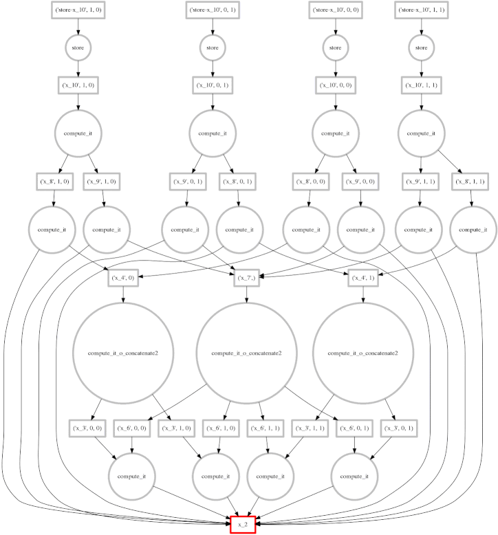
To keep a small memory footprint we avoid holding on to unnecessary intermediate data. The full computation graph of a smaller problem might look like the following:
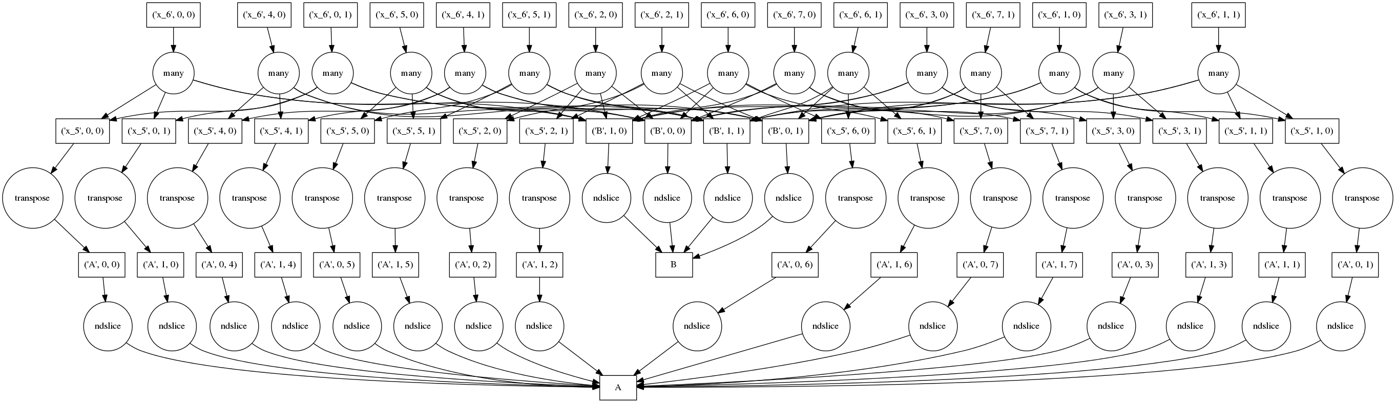
Boxes represent data, circles represent functions that run on that data , arrows specify which functions produce/consume which data.
The top row of circles represent the actual blocked dot products (note the many
data dependence arrows originating from them). The bottom row of circles
represents pulling blocks of data from the the A HDF5 dataset to in-memory
numpy arrays. The second row transposes the blocks from the first row and adds
more blocks from B.
Naively performed, this graph can be very bad; we replicate our data four times here, once in each of the rows. We pull out all of the chunks, transpose each of them, and then finally do a dot product. If we couldn’t fit the original data in memory then there is no way that this will work.
Function Inlining
We resolve this in two ways. First, we don’t cache intermediate values for
fast-running functions (like np.transpose). Instead we inline fast functions
into tasks involving expensive functions (like np.dot).
We may end up running the same quick function twice, but at least we
won’t have to store the result. We trade computation for memory.
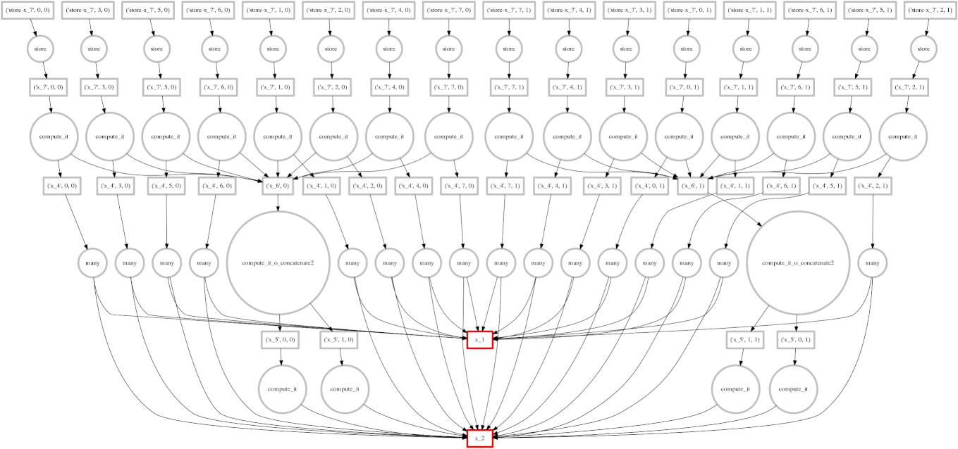
The result of the graph above with all access and transpose operations inlined looks like the following:
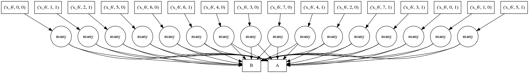
Now our tasks nest (see below). We run all functions within a nested task as a single operation. (non-LISP-ers avert your eyes):
('x_6', 6, 0): (dotmany, [(np.transpose, (ndslice, 'A', (1000, 1000), 0, 6)),
                          (np.transpose, (ndslice, 'A', (1000, 1000), 1, 6))],
                          [(ndslice, 'B', (1000, 1000), 0, 0),
                           (ndslice, 'B', (1000, 1000), 1, 0)]),
This effectively shoves all of the storage responsibility back down to the HDF5 store. We end up pulling out the same blocks multiple times, but repeated disk access is inevitable on large complex problems.
This is automatic. Dask now includes an inline function that does this
for you. You just give it a set of “fast” functions to ignore, e.g.
dsk2 = inline(dsk, [np.transpose, ndslice, add, mul, ...])
Scheduler
Now that we have a nice dask to crunch on, we run those tasks with multiple worker threads. This is the job of a scheduler.
We build and document such a scheduler here. It targets a shared-memory single-process multi-threaded environment. It replaces the elegant 20 line reference solution with a large blob of ugly code filled with locks and mutable state. Still, it manages the computation sanely, performs some critical optimizations, and uses all of our hardware cores (Moore’s law is dead! Long live Moore’s law!)
Many NumPy operations release the GIL and so are highly amenable to multi-threading. NumPy programs do not suffer the single-active-core-per-process limitation of most Python code.
Approach
We follow a fairly standard model. We create a ThreadPool with a fixed
number of workers. We analyze the dask to determine “ready to run” tasks.
We send a task to each of our worker threads. As they finish they update the
run-state, marking jobs as finished, inserting their results into a shared
cache, and then marking new jobs as ready based on the newly available data.
This update process is fully indexed and handled by the worker threads
themselves (with appropriate locks) making the overhead negligible and
hopefully scalable to complex workloads.
When a newly available worker selects a new ready task they often have several to choose from. We have a choice. The choice we make here is very powerful. The next section talks about our selection policy:
Select tasks that immediately free data resources on completion
Optimizations
Our policy to prefer tasks that free resources lets us run many computations in a very small space. We now show three expressions, their resulting schedules, and an animation showing the scheduler walk through those schedules. These were taken from live runs.
Example: Embarrassingly parallel computation
On the right we show an animated GIF of the progress of the following embarrassingly parallel computation:
expr = (((A + 1) * 2) ** 3)
Circles represent computations, boxes represent data.
Red means actively taking up resources. Red is bad.
- Red circles: tasks currently executing in a thread
- Red boxes: data currently residing in the cache occupying precious memory
Blue means finished or released. Blue is good.
- Blue circles: finished tasks
- Blue boxes: data released from memory because we no longer need it for any task
We want to turn all nodes blue while minimizing the number of red boxes we have at any given time.
The policy to execute tasks that free resources causes “vertical” execution when possible. In this example our approach is optimal because the number of red boxes is kept small throughout the computation. We have one only red box for each of our four threads.
Example: More complex computation with Reductions
We show a more complex expression:
expr = (B - B.mean(axis=0)) + (B.T / B.std())
This extends the class of expressions that we’ve seen so far to reductions and
reductions along an axis. The per-chunk reductions start at the bottom and
depend only on the chunk from which they originated. These per-chunk results
are then concatenated together and re-reduced with the large circles (zoom in
to see the text concatenate in there.) The next level takes these (small)
results and the original data again (note the long edges back down the bottom
data resources) which result in per-chunk subtractions and divisions.
From there on out the work is embarrassing, resembling the computation above. In this case we have relatively little parallelism, so the frontier of red boxes covers the entire image; fortunately the dataset is small.
Example: Fail Case
We show a case where our greedy solution fails miserably:
expr = (A.T.dot(B) - B.mean(axis=0))
The two large functions on the second level from the bottom are the computation
of the mean. These are cheap and, once completed,
allow each of the blocks of the dot product to terminate quickly and release
memory.
Tragically these mean computations execute at the last possible moment,
keeping all of the dot product result trapped in the cache.
We have almost a full row of red boxes at one point in the computation.
In this case our greedy solution was short sighted; a slightly more global solution would quickly select these large circles to run quickly. Perhaps betweenness centrality would resole this problem.
On-disk caching
We’ll never build a good enough scheduler. We need to be able to fall back to on-disk caching. Actually this isn’t terrible. High performance SSDs get close to 1 GB/second throughput and in the complex cases where data-aware scheduling fails we probably compute slower than that anyway.
I have a little disk-backed dictionary project,
chest, for this but it’s immature. In
general I’d like to see more projects implement the dict interface with
interesting policies.
Trouble with binary data stores
I have a confession, the first computation, the very large dot product, sometimes crashes my machine. While then scheduler manages memory well I have a memory leak somewhere. I suspect that I use HDF5 improperly.
I also tried doing this with bcolz. Sadly nd-chunking is not well
supported. email thread
here and
here.
Expression Scope
Blaze currently generates dasks for the following:
- Elementwise operations (like
+,*,exp,log, …) - Dimension shuffling like
np.transpose - Tensor contraction like
np.tensordot - Reductions like
np.mean(..., axis=...) - All combinations of the above
We also comply with the NumPy API on these operations.. At the time of writing notable missing elements include the following:
- Slicing (though this should be easy to add)
- Solve, SVD, or any more complex linear algebra. There are good solutions to this implemented in other linear algebra software (Plasma, Flame, Elemental, …) but I’m not planning to go down that path until lots of people start asking for it.
- Anything that NumPy can’t do.
I’d love to hear what’s important to the community. Re-implementing all of NumPy is hard, re-implementing a few choice pieces of NumPy is relatively straightforward. Knowing what those few choices pieces are requires community involvement.
Bigger ideas
My experience building dynamic schedulers is limited and my approach is likely suboptimal. It would be great to see other approaches. None of the logic in this post is specific to Blaze or even to NumPy. To build a scheduler you only need to understand the model of a graph of computations with data dependencies.
If we were ambitious we might consider a distributed scheduler to execute these task graphs across many nodes in a distributed-memory situation (like a cluster). This is a hard problem but it would open up a different class of computational solutions. The Blaze code to generate the dasks would not change ; the graphs that we generate are orthogonal to our choice of scheduler.
Help
I could use help with all of this, either as open source work (links below) or for money. Continuum has funding for employees and ample interesting problems.
Links:
blog comments powered by Disqus